Getting Started with momst
Jorge A. Parraga-Alava
2026-06-02
Source:vignettes/getting-started.Rmd
getting-started.RmdOverview
The momst package solves the Multi-Objective Minimum Spanning Tree (MO-MST) problem on complete weighted graphs. Given a graph where every edge carries two or three independent costs (for example: distance, time, and risk), the goal is to obtain the Pareto front of spanning trees that no other tree dominates in all objectives simultaneously.
The solver is built around the NSGA-II algorithm
(Non-dominated Sorting Genetic Algorithm II) and uses Prufer
sequences as the chromosome representation. By Cayley’s
theorem, every integer vector of length n - 2 with values
in {1, ..., n} decodes to a unique spanning tree of
n nodes, so the representation is closed under random
sampling, crossover, and mutation. This avoids the need for any repair
operator.
The package exposes four solver variants that differ in the local search operator applied after each generation:
| Variant | Local search |
|---|---|
"base" |
None (pure NSGA-II) |
"PR" |
Path Relinking |
"PLS" |
Pareto Local Search |
"TS" |
Tabu Search |
This vignette shows the minimal workflow:
- Generate a random instance.
- Run
run_momst()with a chosen variant. - Inspect the population, the per-iteration Pareto fronts, and the global Pareto front.
- Visualise the global Pareto front and the best-compromise spanning tree.
A companion vignette
(vignette("momst-variants", package = "momst")) compares
the four variants side by side.
Reference
This package is the reference implementation of the method described in:
Parraga-Alava, J., Inostroza-Ponta, M., and Dorn, M. (2017). “Using local search strategies to improve the performance of NSGA-II for the Multi-Criteria Minimum Spanning Tree problem”. In 2017 IEEE Congress on Evolutionary Computation (CEC), pages 1818 to 1825. IEEE. doi:10.1109/CEC.2017.7969432
To get the citation entry from within R:
citation("momst")Installation
You can install the development version of the package directly from GitHub:
# install.packages("remotes")
remotes::install_github("jorgeklz/momst", build_vignettes = TRUE)A first end-to-end example
Step 1. Generate a random bi-objective instance
generate_instance() returns an edge list of a complete
graph with random uniform weights for every objective. The
seed argument makes the instance fully reproducible without
polluting the global random number generator.
# Number of nodes and number of objectives
n_nodes   <- 10
n_obj     <- 2

# Generate a complete graph with two independent weights per edge
inst <- generate_instance(
  n        = n_nodes,
  num_obj  = n_obj,
  range_a  = c(10, 100),   # weight range for objective 1
  range_b  = c(10,  50),   # weight range for objective 2
  seed     = 12345
)

# The instance has n*(n-1)/2 edges
nrow(inst)
#> [1] 45

# First six edges of the complete graph
head(inst)
#>   from to weight_1 weight_2
#> 1    1  2 74.88135 22.84899
#> 2    1  3 88.81959 12.40781
#> 3    1  4 78.48841 11.73826
#> 4    1  5 89.75121 12.20215
#> 5    1  6 51.08329 35.02171
#> 6    1  7 24.97346 48.57881
For performance, the package converts the edge list into one
n x n lookup matrix per objective so that the cost of any
edge (i, j) can be retrieved in constant time:
lk <- build_weight_lookup(inst, n_nodes, n_obj)

# Each element is a symmetric weight matrix
str(lk, max.level = 1)
#> List of 2
#>  $ : num [1:10, 1:10] 0 74.9 88.8 78.5 89.8 ...
#>  $ : num [1:10, 1:10] 0 22.8 12.4 11.7 12.2 ...

# Weight of edge (1, 2) in objective 1
lk[[1]][1, 2]
#> [1] 74.88135
Step 2. Run the NSGA-II solver (base variant)
run_momst() is the main entry point. It performs:
-
iterationsindependent runs of NSGA-II (useful to average results). - Inside each run, up to
max_generationsevolutionary cycles. - After every cycle, a local search operator is applied to the current
non-dominated set (none for
"base"). - A global Pareto front is assembled from the final population of each independent run.
For a first contact we use the simplest variant, "base".
A small instance and short runs are enough to illustrate the
workflow.
res_base <- run_momst(
  instance        = inst,
  n               = n_nodes,
  num_obj         = n_obj,
  variant         = "base",      # pure NSGA-II
  iterations      = 3,           # three independent runs
  pop_size        = 30,          # must be even
  tour_size       = 2,           # binary tournament selection
  cross_rate      = 0.80,        # crossover probability
  mut_rate        = 0.10,        # per-individual mutation probability
  max_generations = 40,          # generations per run
  convergence_window = 8,        # early stopping window
  verbose         = FALSE,
  seed            = 2026
)
The function returns a list with everything needed to analyse the results:
names(res_base)
#> [1] "instance"        "lookup"          "iterations"      "pareto_per_iter"
#> [5] "global_pareto" "elapsed"-
instance: the edge list used. -
lookup: the per-objective weight matrices. -
iterations: the final populations of every independent run. -
pareto_per_iter: the Pareto front of every independent run. -
global_pareto: the non-dominated union of all those fronts. -
elapsed: wall-clock time in seconds.
Step 3. Inspect the global Pareto front
Each row of global_pareto is a candidate spanning tree.
The first n - 2 columns are the Prufer sequence (the
chromosome), and the columns objective_1,
objective_2 (and optionally objective_3)
report the total cost of the tree in each
objective.
# Number of non-dominated trees
nrow(res_base$global_pareto)
#> [1] 17

# Show the chromosomes and their objective values
res_base$global_pareto
#>       V1 V2 V3 V4 V5 V6 V7 V8 objective_1 objective_2 rankingIndex    density
#> X.16   7  5  2 10  7  2  4  9    249.3887    247.8416            1        Inf
#> X      3  7 10 10  7  2  4 10    380.7875    155.4644            1        Inf
#> X.251  7  7 10 10  7  2  4  9    293.7133    203.1376            1 0.19957716
#> X.151 10  7 10 10  7  2  4  9    344.2333    173.0798            1 0.16530635
#> X.131  8  7 10 10  7  2  4  9    307.9984    197.6509            1 0.16149706
#> X.12   7  7 10 10  7  2  4 10    316.9414    191.6354            1 0.16149706
#> X.21   3  7 10 10  7  2  4  9    357.5594    166.9666            1 0.16149706
#> X.24  10  7 10 10  7  2  4 10    367.4614    161.5776            1 0.16149706
#> X.17   8  7  8 10  7  2  4  9    291.5831    217.8454            1 0.14951032
#> X.19   7  5 10 10  7  2  4  9    268.9845    224.6546            1 0.14951032
#> X.5    8  7 10 10  7  2  4 10    331.2265    186.1487            1 0.14935738
#> X.29   8  5  8 10  7  2  4  9    266.8543    239.3624            1 0.14364817
#> X.301 10  5 10 10  7  2  4 10    342.7326    183.0947            1 0.13737064
#> X.261  8  5  2 10  7  2  4  9    263.6738    242.3549            1 0.08808047
#> X.4    7  5  8 10  7  2  4  9    252.5692    244.8491            1 0.08808047
#> X.361  7  7  8 10  7  2  4  9    277.2980    223.3321            1 0.08808047
#> X.31   8  5 10 10  7  2  4  9    283.2696    219.1679            1 0.08808047
We can sort the front by objective 1 to see the typical trade-off between objectives:
front <- res_base$global_pareto[order(res_base$global_pareto$objective_1), ]
front[, c("objective_1", "objective_2")]
#>       objective_1 objective_2
#> X.16     249.3887    247.8416
#> X.4      252.5692    244.8491
#> X.261    263.6738    242.3549
#> X.29     266.8543    239.3624
#> X.19     268.9845    224.6546
#> X.361    277.2980    223.3321
#> X.31     283.2696    219.1679
#> X.17     291.5831    217.8454
#> X.251    293.7133    203.1376
#> X.131    307.9984    197.6509
#> X.12     316.9414    191.6354
#> X.5      331.2265    186.1487
#> X.301    342.7326    183.0947
#> X.151    344.2333    173.0798
#> X.21     357.5594    166.9666
#> X.24     367.4614    161.5776
#> X        380.7875    155.4644
The “extreme” solutions of the front are the trees that minimise each objective in isolation:
Step 4. Plot the Pareto front
plot_pareto_front() produces a base-graphics scatter of
the non-dominated set. The dashed line connects consecutive points after
sorting by the first objective, which makes the trade-off easy to
read.
plot_pareto_front(res_base)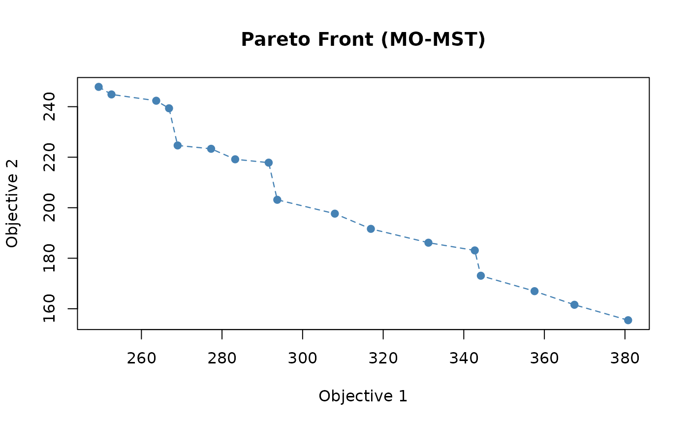
Global Pareto front returned by the base variant.
Step 5. Decode and plot the best-compromise tree
The “best-compromise” tree is the one that minimises the sum of all
objectives. The helper plot_best_tree() decodes its Prufer
chromosome, turns it into an igraph object, and labels each
edge with its cost in every objective.
The igraph package is only needed for this plot; the
rest of the package does not depend on it.
if (requireNamespace("igraph", quietly = TRUE)) {
  plot_best_tree(res_base, n = n_nodes)
} else {
  message("Install 'igraph' to plot the spanning tree.")
}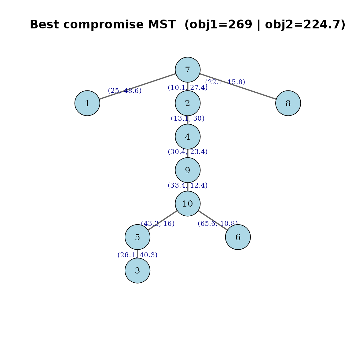
Best-compromise spanning tree of the base variant.
Working with three objectives
The same workflow extends seamlessly to three-objective problems.
Just set num_obj = 3 and supply a third weight range
range_c. The Pareto front then lives in a three-dimensional
objective space.
res_3obj <- run_momst(
  n               = 8,
  num_obj         = 3,
  variant         = "base",
  iterations      = 2,
  pop_size        = 30,
  max_generations = 25,
  range_a         = c(10, 100),
  range_b         = c(10,  50),
  range_c         = c(30, 200),
  verbose         = FALSE,
  seed            = 7
)

# Three-objective non-dominated set
head(res_3obj$global_pareto[, c("objective_1", "objective_2", "objective_3")])
#>       objective_1 objective_2 objective_3
#> X.10     377.2130    105.1852    672.9824
#> X.221    421.0996    114.1803    623.2404
#> X.101    229.8941    155.1778    732.7992
#> X.131    389.0804    189.9002    350.9168
#> X.3      290.4036    204.5720    478.7301
#> X.5      256.0040    135.4129    823.3894
A simple way to inspect the three-objective front without extra dependencies is a pairs plot:
front3 <- res_3obj$global_pareto[, c("objective_1", "objective_2", "objective_3")]
pairs(front3, pch = 19, col = "steelblue")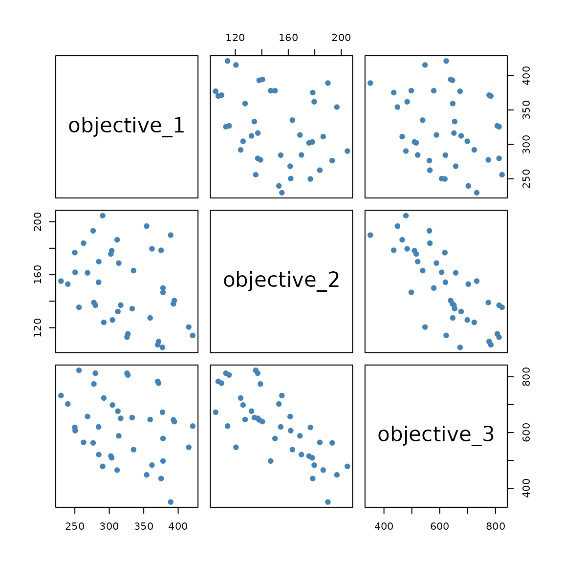
Pairwise projections of the three-objective Pareto front.
Reproducibility
Every stochastic step inside run_momst() is controlled
by the seed argument. Two calls with the same arguments and
the same seed return identical results:
a <- run_momst(n = 8, num_obj = 2, variant = "base",
               iterations = 1, pop_size = 20, max_generations = 15,
               verbose = FALSE, seed = 99)

b <- run_momst(n = 8, num_obj = 2, variant = "base",
               iterations = 1, pop_size = 20, max_generations = 15,
               verbose = FALSE, seed = 99)

identical(a$global_pareto, b$global_pareto)
#> [1] TRUE
Where to go next
-
vignette("momst-variants", package = "momst")runs the four solver variants on the same instance and compares their Pareto fronts both numerically and visually. -
?run_momstdocuments every argument of the main solver. -
?plot_pareto_frontand?plot_best_treedocument the plotting helpers. -
?apply_local_searchdocuments the dispatcher used internally to call the local search operator selected by thevariantargument.